“Let us listen to our cities. Is it not the very nature of the urban environment to make us hear, whether we like it or not, the mixing of sounds?”

Jean-Francois Augoyard, Henry Torque, Sonic Experience - A Guide to Everyday Sounds (2005)

Every urban design plan has its own sound signature unique with its sonic environment. I used to discover sound records from the radio, street, the club lineups or the public events, coffee shops, however, often the origin of the music remains unknown. The soundscape from the cities characterises the culture just as any languages identified within a context of a given origin and time.

Today sound recognition algorithms identifies plagiarism in music, controls licensing, and help discovering who was the initial inspiration to some pioneers across different genres in classical music, pop, jazz and others. Engineer Jovan Jovanovic explains in this article how this algorithm works in Shazam, the world’s premier audio recognition. The Shazam app has been downloaded more than 500 million times and has over 100 million monthly active users.

As an alternative to mobile app RapidAPI provides the largest Web API hub with similar or identical services available for commercial and non-commercial use for engineers.

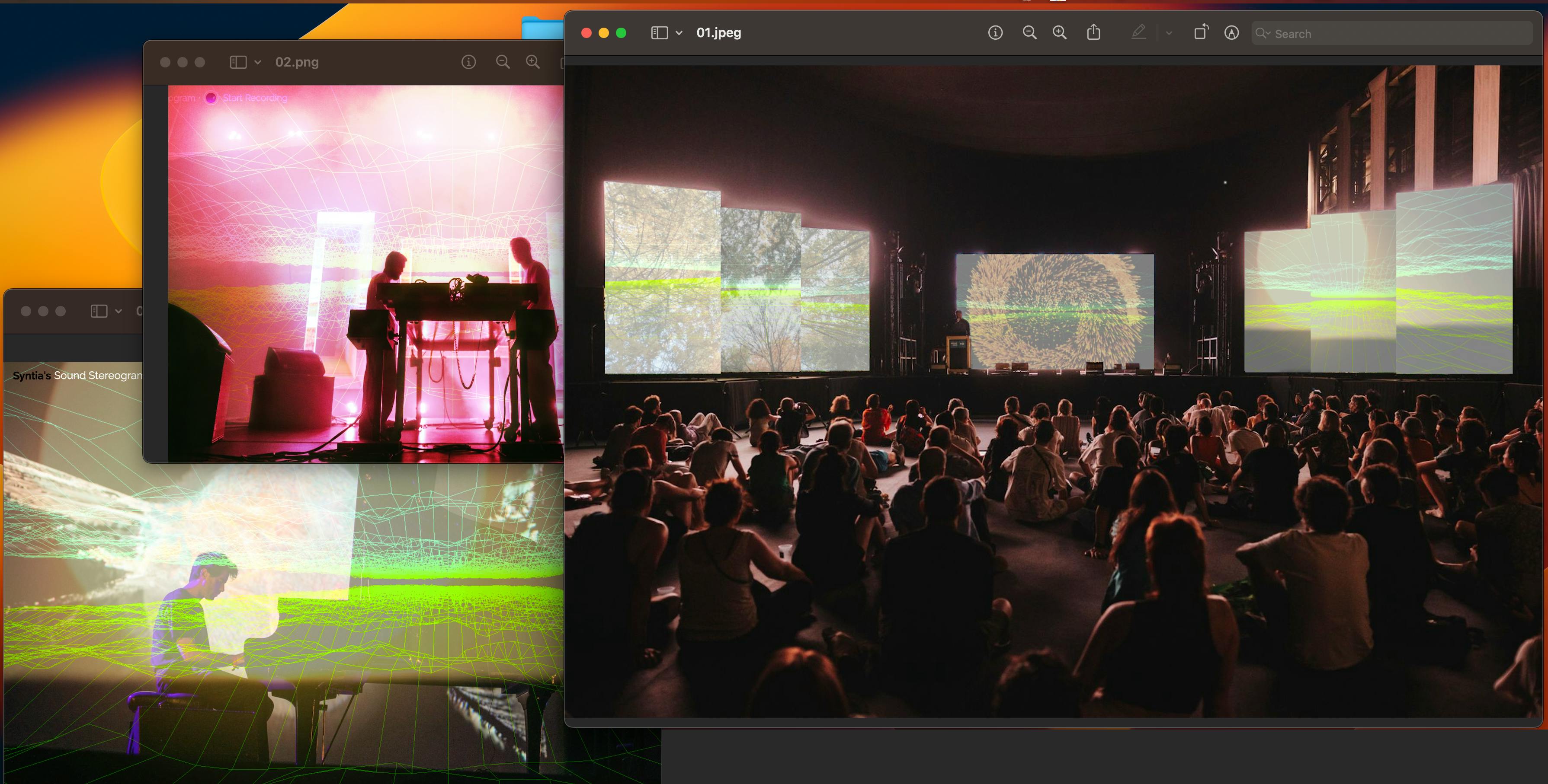
Aggregating APIs for sound recording, song recognition and search on Spotify I discovered the essential services for maximising the sound listening experience and discovery. “Syntia’s Sound Stereograph” is a web software available to record sounds, discover the artists and their work. I’m awaiting the final acceptance from Spotify before the first official launch. Meanwhile I’m working on the visual rendering to adapt the sound input and processing.

Visualising the frequency domain on the 3D plot has an immersive effect with visual “stereograph”- data responding on sound frequencies. This web platform doesn’t require the application on device and is suitable for streaming sound performances and creating a unique listenting experiences.

Audio Stereograph preview:

Digital signal processing in sound recognition

Modern device’s built-in audio signal processing allows us to recognize sounds with an algorithms. If you record a short version of a song it will create a fingerprint for the recorded sample, lookup the database and use its music recognition algorithm to tell you exactly which song you are listening to.

In a microphone, the first electrical component to encounter this signal translates it into an analog voltage signal. The continuous signal is being processed into a discrete signal that can be stored digitally. It is done by capturing a digital value that represents the amplitude of the signal.

The conversion involves quantization of the input, and it necessarily introduces a small amount of error. Therefore, instead of a single conversion, an analog-to-digital converter performs many conversions on very small pieces of the signal - a process known as sampling.

The Nyquist–Shannon sampling theorem

The Nyquist–Shannon sampling theorem is an essential principle for digital signal processing linking the frequency range of a signal and the sample rate required to avoid a type of distortion called aliasing.

The sampling theorem states that the sample rate must be at least twice the bandwidth of the signal to avoid aliasing distortion. In particular, to capture all of the frequencies that a human can hear in an audio signal, we must must sample the signal at a frequency twice that of the human hearing range.

The human ear can detect frequencies roughly between 20 Hz and 20,000 Hz. As a result, audio is most often recorded at a sampling rate of 44,100 Hz. This is the sampling rate commonly used for lossy compression to MPEG-1 and VCD, SVCD and MP3 audio and video formats.

Recording a sampled audio signal

The modern soundcards has build-in analog-to-digital converters. Software for sound recording are build with programming languages such as Java, Python, and sound processing libraries,- setting the frequency of the sample, number of channels mono or stereo, and sample size such as 16 or 24 bit samples. Then by opening the line from your sound card start writing to a byte array. Here is an example how it can be done in Java by reading the data from TargetDataLine:

private AudioFormat getFormat() {
    float sampleRate = 44100;
    int sampleSizeInBits = 16;
    int channels = 1;          //mono
    boolean signed = true;     //Indicates whether the data is signed or unsigned
    boolean bigEndian = true;  //Indicates whether the audio data is stored in big-endian or little-endian order
    return new AudioFormat(sampleRate, sampleSizeInBits, channels, signed, bigEndian);
}

final AudioFormat format = getFormat(); //Fill AudioFormat with the settings
DataLine.Info info = new DataLine.Info(TargetDataLine.class, format);
final TargetDataLine line = (TargetDataLine) AudioSystem.getLine(info);
line.open(format);
line.start();

In following example, the running flag is a global variable which is stopped by another thread, interface with the “Stop” button.

OutputStream out = new ByteArrayOutputStream();
running = true;

try {
    while (running) {
        int count = line.read(buffer, 0, buffer.length);
        if (count > 0) {
            out.write(buffer, 0, count);
        }
    }
    out.close();
} catch (IOException e) {
    System.err.println("I/O problems: " + e);
    System.exit(-1);
}

Fourier series

What we have in this byte array is signal recorded in the time domain. The time-domain signal represents the amplitude change of the signal over time.

In the early 1800s, Jean-Baptiste Joseph Fourier made the remarkable discovery that any signal in the time domain is equivalent to the sum of some possibly infinite number of simple sinusoidal signals, given that each component sinusoid has a certain frequency, amplitude, and phase. The series of sinusoids that together form the original time-domain signal is known as its Fourier series.

This representation of the signal is known as the frequency domain. In some ways, the frequency domain acts as a type of fingerprint or signature for the time-domain signal, providing a static representation of a dynamic signal.

The following animation demonstrates the Fourier series of a 1 Hz square wave, and how an approximate square wave can be generated out of sinusoidal components. The signal is shown in the time domain above, and the frequency domain below.

Analyzing a signal in the frequency domain simplifies many things immensely. It is more convenient in the world of digital signal processing because the engineer can study the spectrum (the representation of the signal in the frequency domain) and determine which frequencies are present, arrange or filter them to reconstruct the tone.

The Discrete Fourier Transform

The process of converting signal from the time to the frequency domain does Discrete Fourier Transform (DFT). The DFT is a mathematical methodology for performing Fourier analysis on a discrete sampled signal. It converts a finite list of equally spaced samples of a function into the list of coefficients of a finite combination of complex sinusoids, ordered by their frequencies, by considering if those sinusoids had been sampled at the same rate.

One of the well known numerical algorithms for the calculation of DFT is the Fast Fourier transform (FFT) with variation of FFT Cooley–Tukey algorithm. This is a divide-and-conquer algorithm that recursively divides a DFT into many smaller DFTs. Whereas evaluating a DFT directly requires O(_n_2) operations, with a Cooley-Tukey FFT the same result is computed in O(n log n) operations.

The FFT supports many programming languages, for example in C FFTW, C++ EigenFFT, Java JTransform, Python NumPy, Ruby Ruby-FFTW3 (Interface to FFTW).

Below is an example of an FFT function written in Java. (FFT takes complex numbers as input. To understand the relationship between complex numbers and trigonometric functions, read about Euler’s formula.)

public static Complex[] fft(Complex[] x) {
    int N = x.length;
    
    Complex[] even = new Complex[N / 2];
    for (int k = 0; k < N / 2; k++) {
        even[k] = x[2 * k];
    }
    Complex[] q = fft(even);

    Complex[] odd = even; // reuse the array
    for (int k = 0; k < N / 2; k++) {
        odd[k] = x[2 * k + 1];
    }
    Complex[] r = fft(odd);

    Complex[] y = new Complex[N];
    for (int k = 0; k < N / 2; k++) {
        double kth = -2 * k * Math.PI / N;
        Complex wk = new Complex(Math.cos(kth), Math.sin(kth));
        y[k] = q[k].plus(wk.times(r[k]));
        y[k + N / 2] = q[k].minus(wk.times(r[k]));
    }
    return y;
}

And here is an example of a signal before and after FFT analysis:

Audio identification

One unfortunate side effect of FFT is that we lose a great deal of information about timing. For a timing a buffer is neede transform just this part of the information. The size of each chunk can be determined in a different ways.

In example for a sound recorded in stereo with 16-bit samples at 44,100 Hz, one second of such chunk will be 44,100 samples * 2 bytes * 2 channels ≈ 176 kB. With a 4 kB for the size we will have 44 chunks of data to analyze in every second of the song.

byte audio [] = out.toByteArray()
int totalSize = audio.length
int sampledChunkSize = totalSize/chunkSize;
Complex[][] result = ComplexMatrix[sampledChunkSize][];

for(int j = 0;i < sampledChunkSize; j++) {
  Complex[chunkSize] complexArray;

  for(int i = 0; i < chunkSize; i++) {
    complexArray[i] = Complex(audio[(j*chunkSize)+i], 0);
  }

  result[j] = FFT.fft(complexArray);
}

In the inner loop the time-domain data (the samples) hsd a complex number with imaginary part 0. The outer loop iterates through the chunks and performs FFT analysis on each.

Once the frequency data of the signal is collected, the main challenge is how to distinguish which frequencies are the most important in recognition process. Intuitively, we search for the frequencies with the highest magnitude or peaks.

In one song the range of frequencies might vary between low C - C1 32.70 Hz and high C - C8 4,186.01 Hz interval. Instead of analyzing the entire frequency range at once, comparing several smaller intervals based on the common frequencies and analyze each separately is more efficient, because it allocates less memory to store the data.

In example of Shazam’s algorithm these are 30 Hz - 40 Hz, 40 Hz - 80 Hz and 80 Hz - 120 Hz for the low tones when covering bass guitar, and 120 Hz - 180 Hz and 180 Hz - 300 Hz for the middle and higher tones when covering vocals and most other instruments.

Identifying the frequency with the highest magnitude within each interval forms a signature for this chunk of the song, and this signature becomes part of the fingerprint of the song.

public final int[] RANGE = new int[] { 40, 80, 120, 180, 300 };

// find out in which range is frequency
public int getIndex(int freq) {
    int i = 0;
    while (RANGE[i] < freq)
        i++;
    return i;
}
    
// result is complex matrix obtained in previous step
for (int t = 0; t < result.length; t++) {
    for (int freq = 40; freq < 300 ; freq++) {
        // Get the magnitude:
        double mag = Math.log(results[t][freq].abs() + 1);

        // Find out which range we are in:
        int index = getIndex(freq);

        // Save the highest magnitude and corresponding frequency:
        if (mag > highscores[t][index]) {
            points[t][index] = freq;
        }
    }
    
    // form hash tag
    long h = hash(points[t][0], points[t][1], points[t][2], points[t][3]);
}

private static final int FUZ_FACTOR = 2;

private long hash(long p1, long p2, long p3, long p4) {
    return (p4 - (p4 % FUZ_FACTOR)) * 100000000 + (p3 - (p3 % FUZ_FACTOR))
            * 100000 + (p2 - (p2 % FUZ_FACTOR)) * 100
            + (p1 - (p1 % FUZ_FACTOR));
}

A fuzz factor is system of analysis based on the quality of recording, i.e. when the recording isn’t done perfectly. This signature becomes the key in a hash table. The corresponding value is the time this set of frequencies appeared in the song, along with the song ID (song title and artist). Here’s an example of how these records might appear in the database.

Hash Tag	Time in Seconds	Song
30 51 99 121 195	53.52	Song A by artist A
33 56 92 151 185	12.32	Song B by artist B
39 26 89 141 251	15.34	Song C by artist C
32 67 100 128 270	78.43	Song D by artist D
30 51 99 121 195	10.89	Song E by artist E
34 57 95 111 200	54.52	Song A by artist A
34 41 93 161 202	11.89	Song E by artist E

Based on this music identification process it is possible to create a database with a digital fingerprint on every song and use it to identify songs by searching the database for the matching hash tags. Each song also has standard code for uniquely identifying sound recordings and music video recordings (ISRC).

With the multiple matched hashes, the relative timing of the matches can be analysed; therefore increasing the probability of results.

// Class that represents specific moment in a song
private class DataPoint {

    private int time;
    private int songId;

    public DataPoint(int songId, int time) {
        this.songId = songId;
        this.time = time;
    }
    
    public int getTime() {
        return time;
    }
    public int getSongId() {
        return songId;
    }
}

Let’s take i1 and i2 as moments in the recorded song, and j1 and j2 as moments in the song from the database. Probability of the equation from two songs is calculated if recorded sample has identified two hashes in the database and if the subtract interval between two timestamps in song and recording are the same.